What is a Random Number?
Charlie Grover, PhD and Cryptographer at Crypto Quantique, explains what a random number really is, and is it truly random?
Is my random more random than yours: What even is a random number anyway?
Access to a source of random numbers is a necessity for almost all of modern cryptography. We talk regularly about what is a random number and more importantly, when we talk about generating secret keys, we just mean random strings. Ultimately, a key is derived from something called a “seed”, which is just a long string of random bits. Once the seed is determined, it is transformed into a key format, such as the prime numbers used in RSA encryption, using a mathematical algorithm called a Key Derivation Function. For all this to work, we need the seed to be genuinely random, otherwise, there’s no point in building elaborate security algorithms – an attacker who can reverse engineer the seed can just regenerate your private key and circumvent the cryptography instead!
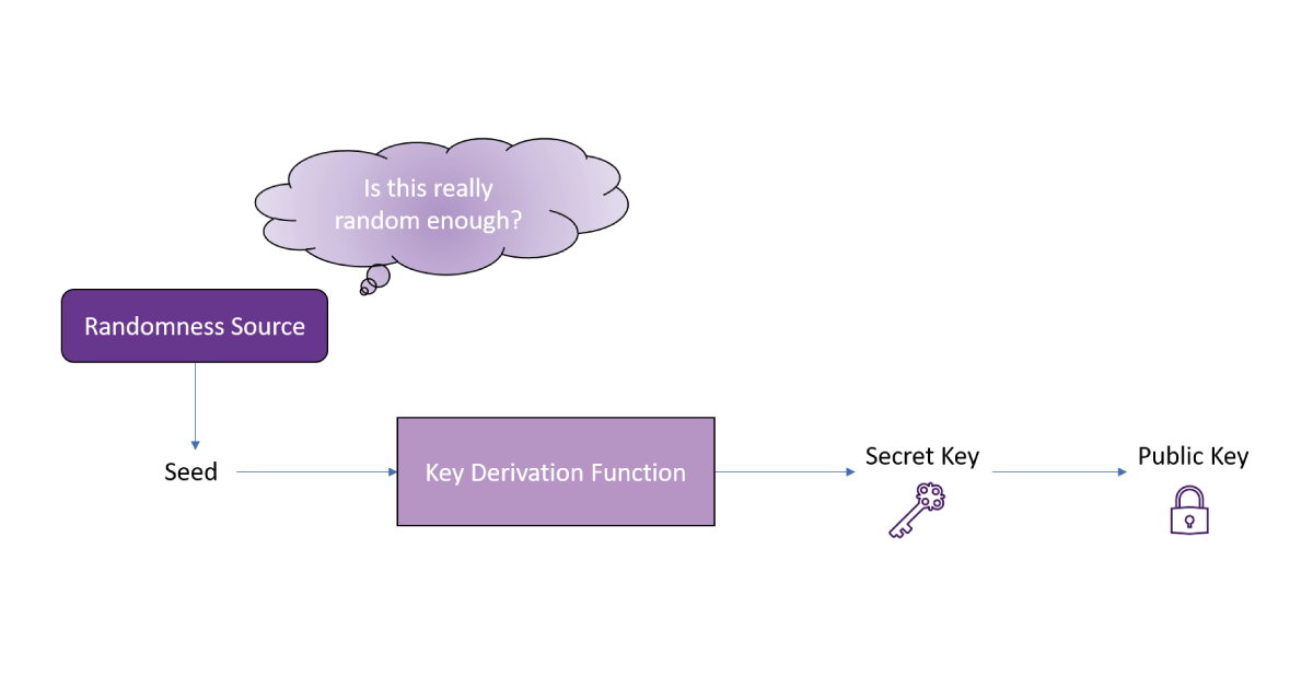
Closer to home, we’ve all become used to being asked for “strong” passwords, obscure looking strings of numbers, letters, and characters that we’re forever doomed to not remember. Of course, there are practical issues with asking people to have a separate random password for every website – it turns out that human brains are not databases and prefer something far more memorable – but these strange passwords do serve a functional purpose. Once you’ve selected your password, an algorithm turns it into a cryptographic key, so for an attacker guessing your password presents a shortcut around any well-built security. If you’re using “thisismypassword” or “qwerty123” for all your accounts, it won’t take an attacker too long to break into them. On the other hand, if you have a meaningless string of characters, it’s quite a lot harder to guess! Incidentally, if you’re struggling to handle the volume of strange-looking passwords you need, consider downloading a password manager to do the heavy lifting for you – they require a single password to use, and generate a “strong” password for each account for you.
These days, some particularly savvy systems use the best of both worlds, asking the user to come up with a ‘random’ sentence by using something ultimately nonsensical – “my pet owl is the Chess world champion” – still hard to guess, but quite memorable in its way. But here arises a key question: how random is random enough? For these human-defined strings, it’s quite hard to decide; I made that last one up off the top of my head, but who’s to say that someone who knows me well enough couldn’t predict what I think is a strange sentence. Mathematically, seeds and secret keys represent numbers, so we can be much more precise. For example, if a password is a string of 10 random letters, there are different possible passwords, or around 100 quadrillions (that’s a 1 followed by fourteen 0s). This requires a lot of guesses, but still way less than is usually considered safe for cryptography. Of course, one can bring in numbers, characters, and case sensitivity to vastly increase the range of passwords, but the point remains – cryptography needs a lot of possibilities. Remember, a seed is just a string of random bits, and the shortest seeds we use in practice typically have length 128 – giving (or a 1 followed by thirty-four 0s) different options to be guessed, so many that even a supercomputer would take billions of years to guess them all.
Is my random more random than yours: What even is a random number anyway?
This might sound like the end of the story – a random seed should be 128 bits long, so if we need something random just make sure it has at least possible outputs. However, the real world isn’t perfect, and if I ask my computer for 128 random bits, can I be sure that it’s generating them truly randomly? The computer can’t exactly toss 128 coins to make the bits, even if we believed that we had access to the world’s most precisely balanced coin. Naïve suggestions such as “just use the date and time” don’t work either – what if an attacker knows my schedule and can predict when I might be generating new account details! Or worse, the metadata on my account could show when it was created. There are many different solutions to the generation of random numbers, enough to fill a blog itself, but most require access to expensive hardware or complex software. In the world of lightweight, embedded devices, this access is unlikely, specialist solutions such as QDID are used, or some randomness is somehow injected during manufacturing. Still, despite all the existing solutions, the question remains: how do we test that the bits we’re using as seed are truly random?
This turns out to be a surprisingly hard question to answer. Intuitively, if we have access to the source of random numbers, we can try to validate that it is a good source experimentally – ask for a lot of output bits and analyse whether or not they look behave like truly random bits should. From this, we can slightly reframe the question to one about the behaviour of random bits: what tests can we devise that random bits should pass, but should detect (possibly subtle) non-random patterns? Remember, non-random data might not be non-random, and a “bad” random number generator might be doing something unremarkably bad, such as every 8th output being the same, rather than just behaving like a biased coin that outputs way more heads than tails.
Let’s have a go ourselves!
It’s part of statistics folklore that human beings are terrible at trying to make random sequences, and almost as bad at distinguishing genuine random sequences from manmade ones. Why is this? Typically, people tend to find that the truly random string doesn’t look random enough, and correspondingly makeup strings that look `extra’ random. Now obviously, statistical tests can tell the difference much better than people can, but understanding why we find it so difficult to do manually can provide some intuition for the kinds of test we want to run. So let’s illustrate this with an example! Below are two random 64-bit strings, one that I made up off the top of my head and one that I generated on my computer using a good source of randomness. Can you work out which one is “real” randomness?
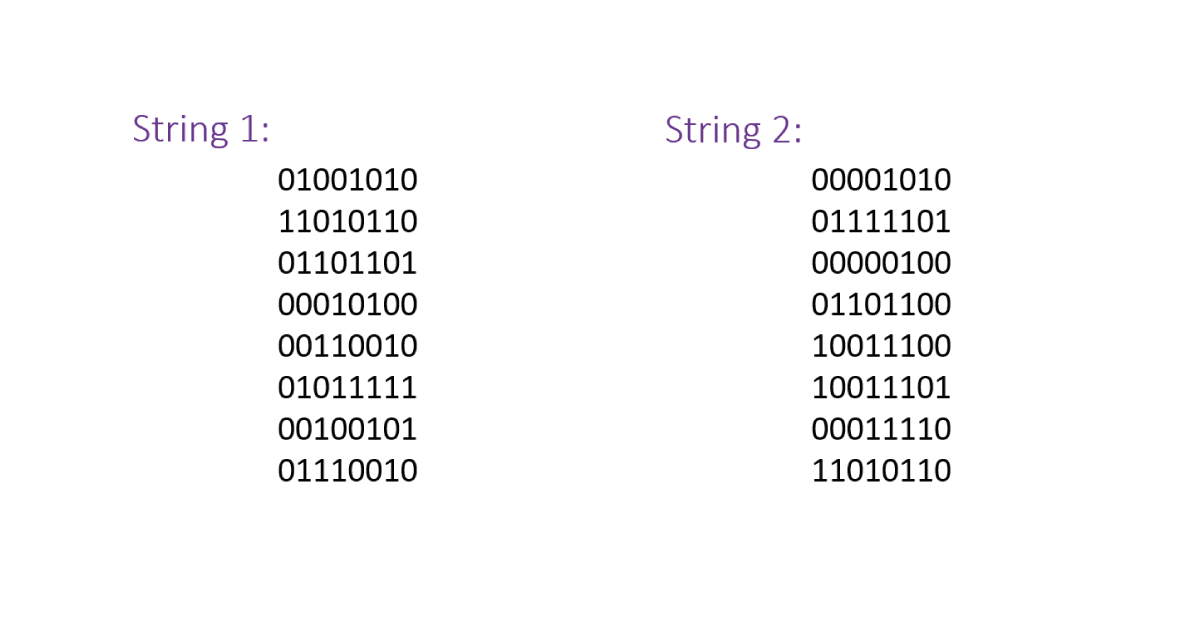
So, how do we go about distinguishing which is which? An obvious place to start is the 0-1 balance of each string – a random string should contain roughly even amounts of both. The first has thirty-three 0s and thirty-one 1s; the second the same. No luck there, and somewhat fortuitous really. Humans tend to have their strings be “too” balanced, when in actuality the odds of getting a perfect 0-1 balance is pretty small, although we would expect something close to an even split. The next thing to look at is the fixed runs in a sequence – continuous runs of 0s or 1s. These appear suspicious to the naked eye, as getting lots of heads on the same coin makes people think it’s weighted. Hence, they don’t appear often in man-made strings but come up more than you might expect in the real world. In a random string of length five, the odds of five 1s is 1/32 (and the same for all 0s). This means we would expect approximately one or two runs of length five of each type to be present in a 64-bit string! In the first string, there’s a run of five 1s, another of four 0s, and everything else has a length of 3 or less. In the second, there’s a run each of five 1s and five 0s, and similarly for length 4 patterns. Here, the first string does not appear to contain enough long runs, but the difference is probably not quite dramatic enough to be conclusive. Still, this measure has been used as a way to root out the fake strings before, such as in The Longest Run of Heads (csun.edu).
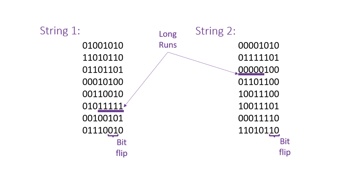
However, my string comes unstuck when we look at a measure humans tend to overestimate: the number of “flips” in the sequence. A flip is when the string changes from a 0 to a 1, or vice versa. For example, 000111 contains just one flip, but 010101 contains five. In general, human-generated strings contain too many flips – our short term memories get uncomfortable when the string doesn’t change quickly enough, and we lose sight of the big picture. On average, there should be around 32 flips in a random string of length 64, since each bit should be different to the previous bit precisely half the time. Looking at our strings, we see that the first string has 39 flips, and the second 31. Here, I’ve been caught out, and we conclude (correctly) that the first string was generated by a human! Whilst this was only a small example, the principles we used to compare the strings can educate the design of proper testing on much more data.
Randomness testing in practice
In the previous example, we distinguished between a real and fake random string by looking at how they behaved compared to how a random string ought to. In the real world, the task is a bit harder – we have to decide whether an individual generator is performing properly or not. Still, this method is a good formula for testing randomness:
- Come up with a handful of tests that check for the `bad’ behaviour of a random number generator.
- Determine how a truly random number generator should perform on these tests.
- Take many independent samples from the generator being tested and see how they compare to the ideal performance.
In general, determining how a random number generator should perform on a test is not too hard. So the difficulty in testing is about determining a sensible collection of tests. Too many tests and things can get a bit cumbersome. Too few, and a bad generator might not be detected. A reasonable method is to come up with a few `natural’ ways that a random number generator could go wrong, and write a test that determines each type of failure. The word natural is slightly subjective here, but one can imagine some common classes of problems: a bad balance of 1s and 0s, over-occurrences of repeating patterns, flipping too often or not often enough, differences between local and global behaviour, and so on. Next time, we will dig into the details of testing a little more. We will take a look at the methodology of common randomness tests, and examine some popular test suits in detail, looking at how they work, when they’re useful, and what behaviours they’re interested in. On the other hand, we will also have a quick look at their limitations – a good design needs more than experimental validation to call something random after all!
We’ve covered a lot in the first part of this blog. We explained the need for good randomness in cryptography, and talked about the challenges around testing for randomness, mostly by comparing a human-generated random string with one from an actual random number generator (RNG). Now we’re going to dive into the technical details a bit more, looking at the mathematics behind the construction of randomness tests, as well as analyzing a popular randomness test suite.
What actually is random?
Before we start talking about testing randomness, we should establish what we mean when we call something random. After all, there are many different kinds of random things in the real world – is it valid to call both a coin flip and a dice roll random? There are more possible outcomes for the dice roll, so intuitively we consider the dice roll to be more random. Conversely, if we only care whether the dice shows an odd or even number, then the amount of randomness we’re interested in should be the same: as with a coin flip, there are exactly two outcomes – an odd or even result – and both are equally likely.
This idea of two equally likely outcomes leads us to the mathematical measure of randomness or uncertainty: Entropy. An event has high entropy if it is hard to predict – for example, when there are lots of possible outcomes that occur with similar likelihood. Conversely, an event has low entropy if it is easy to predict – when some outcomes are much more likely than others, or they’re just aren’t many possible outcomes. The actual unit of entropy is a Bit, defined as the amount of uncertainty in an event with exactly two, equally likely, outcomes. In layman’s terms, that means that an event has one bit of entropy if is equivalent to tossing a fair coin – either a heads or a tails with equal chance. This lets us formalize our notion of a dice roll is more random than a coin flip – the coin flip contains one bit of entropy, but the dice roll contains around 2.6 bits: more than one coin flip, but less than tossing three coins, which has eight equally likely outcomes.
Now, we can properly state the property we are looking for in an RNG: the 128-bit seed output should have exactly 128 bits of entropy, or at least as close to that as physically possible. That is, each bit of the seed should be either a 0 or a 1 with equal chance, and the randomness in each bit should be completely separate from the other ones. This may seem like an obvious statement, but it is important to keep in mind that a bad RNG is probably still outputting something random, just not random enough – and this should fail our tests. This increases the complexity of testing – we’re not just looking to detect random or non-random, rather random enough or not.
Statistical Testing and Sample Sizes
So, how are we going to test an RNG? Although there are tests that try to directly validate the entropy of a random source, it is simpler to resort to statistics and hypothesis tests. These tests take a chunk of output from the RNG analyze some features of the output – such as the balance of 1s and 0s – and consider whether the balance lies in an appropriate region for a true RNG. For example, we might choose an appropriate region so that 99% of the time, the 0-1 balance of a true RNG output would lie in this region. We then test many outputs of the RNG – let’s say 10000 – and see if approximately 1% – or 100 – of the outputs fail. If too many fail, there is evidence that the RNG is skewed towards 0 or 1, thus not producing fair coin flips. However, there’s another possible problem too! If too many pass, there is evidence that the RNG is too consistent, in that it tries to output artificially balanced strings – after all, even a perfect RNG will sometimes output wildly unbalanced strings by chance.
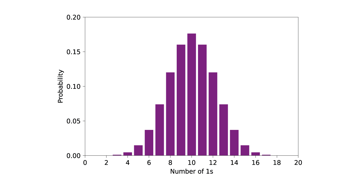
This all sounds a bit abstract, so let’s demonstrate with an example of a small test, in this case examining the 0-1 balance of an RNG. In this example, our RNG –one provided by the NumPy package in python – will output 20 bits at a time, and we say that a string of 20 bits passes if the number of 1s is between 5 and 15, and otherwise the string fails. This range of 1s, between 5 and 15, is the range that the output of a true RNG should lie in around 99% of the time (around 98.8% to be precise). This is calculated by looking at the binomial distribution, as the number of 1s in a 20-bit random string follows the binomial distribution with 20 samples and probability ½. The distribution of 1s should look like the ideal binomial distribution. That is, like this:
Now, let’s take 10000 samples from our RNG and see how it compares:
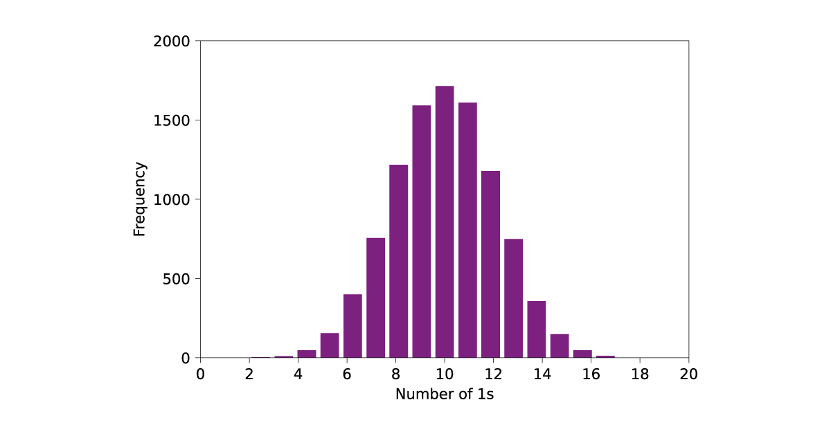
As you can see, the 0-1 balance of the samples lines up well with the predicted binomial distribution. Furthermore, only 142 strings fail the test, around 1.4%, showing that this RNG performs relatively well on this test. What if we had a bad RNG? For example bad RNG, I took 10000 samples from an RNG where each bit is a 0 with a probability of 0.4, and a 1 with a probability of 0.6. That is, equivalent to a coin with a noticeable bias towards 1. The resulting outputs look like this:
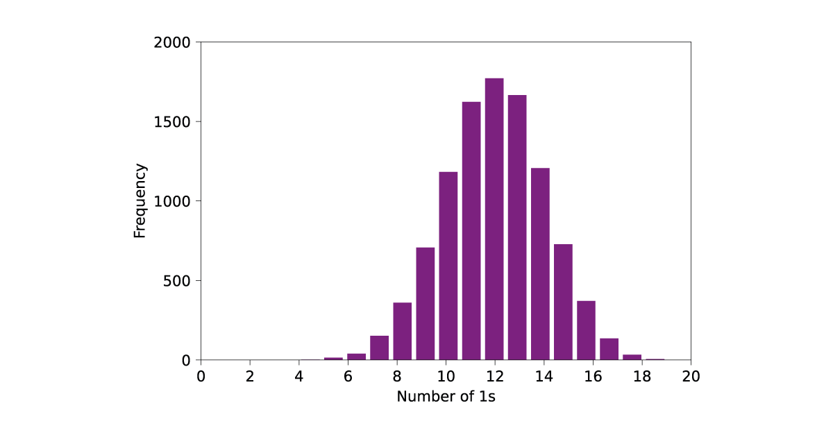
These do not follow the behaviour of a good RNG, as the data is shifted towards having an undesirably large number of 1s. This is demonstrated by the test performance, where 549 of the strings failed the test, quite far from the expected 100. The outcome of these tests tells us what we already knew: our biased RNG is not good, especially when compared to an ideal one. Still, it is random – just lower entropy than an ideal generator. Testing the 0-1 balance is perhaps the simplest test one can imagine, but the same method applies to more complicated tests.
Testing in Practice and the NIST Suite
Now that we’ve seen how randomness tests work, we can move on to what sort of tests are useful. One of the most popular testing suites for an RNG is the NIST (National Institute for Standards and Technology, a U.S. standards body) 800-22 suite,
which defines a sequence of 15 tests for candidate random number generators. As with our example test, each test takes as input many samples – the length varies by test, but imagine each sample as around a million bits long – from the candidate RNG, and grades each sample a pass or a fail. If the proportion of passes matches up well with what we would expect from truly random data, the test indicates no issue with the RNG. Otherwise, there is evidence the RNG is not perfectly random. We can group the tests by looking at what sort of non-randomness NIST is interested in detecting:
- 0-1 Balance: This is examined by the Frequency and Frequency within a Block tests. These tests compare the expected number of 0s and 1s with the actual number, globally within each sample and locally by splitting the sample into smaller sub “blocks”.
- Long Runs: The Runs and Longest-Run-of-Ones in a Block tests check the frequency and length of longest runs on both a global and local scale against the expected amounts.
- Periodic Behaviors: The Maurer’s Universal Statistic and Discrete Fourier Transform tests examine slightly more elaborate periodic features of the output data.
- Template Matching: The Overlapping and Non-Overlapping Template Matching tests consider whether certain pre-defined strings appear as often as expected – if they don’t, there’s evidence the RNG either prefers or avoids certain short patterns.
- Linearity: The Binary Rank Matrix and Linear Complexity tests compare whether or not the output data has linear features that one would not expect from random data, e.g. whether combining previous outputs lets us determine the following ones with some accuracy.
- Bit Flips: The Serial and Approximate Entropy test determine whether the bit string flips appropriately often for random data.
- Deviations Test: The Cumulative Sums and Random Excursions tests consider whether the data tends to drift towards too many 0s or 1s when read in order.
How these tests fit together can be quite hard to understand, and that is part of the problem with randomness testing. It is always hard to justify something as an exhaustive test suite, and it is possible (although unlikely) that a generator may perform well on these tests but have some underlying flaw that an attacker could abuse. Designing them can end up as an exercise in contriving increasingly complicated checks to look for some misbehaviour of a random number generator that none of your existing tests has yet captured.
Best practice: modelling your RNG
The NIST test suite is only one way to test the functionality of a random number generator. Another common one is the DIEHARD suite, which focuses on more general random number generation and less on bit strings. However, regardless of which tests you run, no amount of experimental validation can confirm that an RNG is truly generating random numbers. Instead, any random number generator should be paired with a corresponding mathematical and/or physical model, explaining the methodology of the generation and an analysis of the predicted quality of the output. This is what is required for another NIST test, the 800-90B test, which seeks to estimate the min-entropy of the randomness source, a more conservative measure of randomness than entropy. To qualify for an evaluation under the 800-90B test, the submitter must provide an analytic model of the randomness source, and the analysis affects how the RNG is tested.
This phenomenon cuts both ways; a formal model of a random number generator is insufficient without some experimental data to validate the model. Most random number generation boils down to taking advantage of physical phenomena that are unpredictable given available scientific equipment, often because they occur on a scale that is too small or too fast to analyze using modern techniques. However, the physical effects driving the random number generator may not be suitably random, or may not be measured accurately by the random number generator. For example, anything measured in microelectronics is subject to some amount of noise and unreliability that may dilute the random effects if not carefully considered. Until a random number generator is suitably tested, it is hard to know whether the model lines up well with physical reality. Overall, it is still important to understand how we test randomness, but equally important to keep in mind why – the randomness is necessary to drive cryptography, but cryptography is driven by caution, and just saying that some data passes our test is not cautious enough. Instead, we must use a purpose-built random number generator, whose source of randomness is well-understood and paired with experimental validation that the real-world performance matches up with the model. After all, no amount of good cryptography can provide adequate security without the randomness needed as fuel.
Additional resources
Whitepaper
Enabling Cloud Connectivity in Resource-Constrained IoT Devices: A Wi-Fi Module and Low-End MCU Approach
This paper explores an affordable and efficient approach to embedded device cloud connectivity using a Wi-Fi module with a low-end microcontroller unit…
Read more
Whitepaper
Hardware Root of Trust: QDID PUF & Attopsemi OTP
This whitepaper presents a simplified, secure, and ready-to-use root-of-trust solution for embedded devices by integrating Attopsemi’s I-fuse technology…
Read more
Whitepaper
QuarkLink for Industrial PCs
This white paper introduces how Crypto Quantique’s QuarkLink SaaS device security platform is used with industrial PCs running Linux.
Read more

